Standard input file for geometry optimization
[Show/hide]
%chk=ptch2ar.chk
#p ub3lyp/Def2TZVPP EmpiricalDispersion=GD3 pop=full opt=(CalcAll,MaxCycle=100,MaxStep=100) scf=(MaxConventionalCycles=500)

Pt-CH2-Ar 2-A'

1 2
Pt                    0.69628   1.53758   0.94059
 C                     1.3573    1.45899  -0.52183
 H                     1.45129   0.51482  -1.01643
 H                     1.70351   2.35081  -1.0011
 Ar                    2.66909   1.30611   1.52311

--Link1--
%chk=ptch2ar.chk
#p ub3lyp/Def2TZVPP EmpiricalDispersion=GD3 pop=full opt=(CalcAll) Geom=Check Guess=Read freq(hpmodes) iop(7/33=1)

Pt-CH2-Ar 2-A'

1 2
Specifying a non-standard basis set
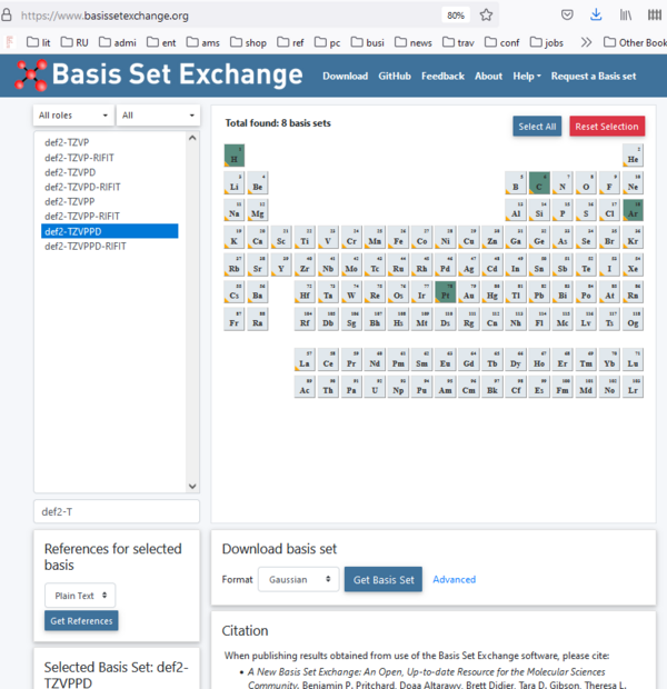
- Find you explicit basis set at the Basis Set Exchange
- Select the basis set and elements you require (Screenshots hidden)
[Show/hide]
- Once you click the 'Get basis set' button, a new page opens with the basis set as you requested
[Show/hide]
- Copy the resulting textbox and enter it in your file, which should look something like this:
[Show/hide]
%chk=ptch2-2ap-d3-tzvppd.chk
#opt b3lyp/gen pseudo=read empiricaldispersion=GD3

Pt-CH2 with a Basis set exchange retrieved basis set

1 2
Pt       0.000000000      0.000000000      0.127324870
C        0.000000000      0.000000000     -1.690790130
H        0.939249500      0.000000000     -2.249590130
H       -0.939249500      0.000000000     -2.249590130

H     0
S   3   1.00
     34.0613410              0.60251978D-02
      5.1235746              0.45021094D-01
      1.1646626              0.20189726
S   1   1.00
      0.32723041             1.0000000
S   1   1.00
      0.10307241             1.0000000
P   1   1.00
      1.40700000             1.0000000
P   1   1.00
      0.38800000             1.0000000
P   1   1.00
      0.95774129632D-01      1.0000000
D   1   1.00
      1.05700000             1.0000000
****
C     0
S   6   1.00
  13575.3496820              0.22245814352D-03
   2035.2333680              0.17232738252D-02
    463.22562359             0.89255715314D-02
    131.20019598             0.35727984502D-01
     42.853015891            0.11076259931
     15.584185766            0.24295627626
S   2   1.00
      6.2067138508           0.41440263448
      2.5764896527           0.23744968655
S   1   1.00
      0.57696339419          1.0000000
S   1   1.00
      0.22972831358          1.0000000
S   1   1.00
      0.95164440028D-01      1.0000000
S   1   1.00
      0.48475401370D-01      1.0000000
P   4   1.00
     34.697232244            0.53333657805D-02
      7.9582622826           0.35864109092D-01
      2.3780826883           0.14215873329
      0.81433208183          0.34270471845
P   1   1.00
      0.28887547253           .46445822433
P   1   1.00
      0.10056823671           .24955789874
D   1   1.00
      1.09700000             1.0000000
D   1   1.00
      0.31800000             1.0000000
D   1   1.00
      0.90985336424D-01      1.0000000
F   1   1.00
      0.76100000             1.0000000
****
Pt     0
S   3   1.00
     30.000000000            0.27148263900
     27.000000000           -0.42226758774
     14.408318564            0.44361581995
S   1   1.00
      5.5335788010           1.0000000
S   1   1.00
      1.2986438223           1.0000000
S   1   1.00
      0.58759393108          1.0000000
S   1   1.00
      0.13845587261          1.0000000
S   1   1.00
      0.49204459888D-01      1.0000000
P   4   1.00
     15.500000000           -0.15672718629
     14.000000000            0.23853412989
      6.1161212339          -0.31041379733
      1.5715586385           0.56473525089
P   1   1.00
      0.75132510781          1.0000000
P   1   1.00
      0.33306466812          1.0000000
P   1   1.00
      0.57000000000D-01      1.0000000
P   1   1.00
      0.20441532514D-01      1.0000000
D   4   1.00
      8.3207937611           0.62945798646D-01
      7.4207226520          -0.90271847072D-01
      1.6570410639           0.16812526416
      0.73943569960          0.25045416970
D   1   1.00
      0.30510856008          1.0000000
D   1   1.00
      0.11350405268          1.0000000
F   1   1.00
      1.3077100              1.0000000
F   1   1.00
      0.4263000              1.0000000
G   1   1.00
      1.0162300              1.0000000
****

PT     0
PT-ECP     3     60
f potential
  1
2      3.30956857            24.31437573
s-f potential
  3
2     13.42865130           579.22386092
2      6.71432560            29.66949062
2      3.30956857           -24.31437573
p-f potential
  3
2     10.36594420           280.86077422
2      5.18297210            26.74538204
2      3.30956857           -24.31437573
d-f potential
  3
2      7.60047949           120.39644429
2      3.80023974            15.81092058
2      3.30956857           -24.31437573
- Note the extra empty lines, Gaussian can be very picky
Restarting an unfinished job
Copy the checkpointfile, or re-use the old one. Then use the keywords Geom=Check Guess=Read opt freq
Trouble with SCF convergence
Use the keywords Geom=Check Guess=Read scf=qc opt freq
Transition dipole moments
Get the derivatives of the dipole moment wrt the normal coordinates by using the Freq=PrintDerivatives keyword:
#p ub3lyp/Def2TZVPP Geom=Check Guess=Read freq(hpmodes,PrintDerivatives)
If you first want to enusre a proper optimalization, split the job in two, and add a second job:
--Link1--
%chk=ptch2v2.chk
#p ub3lyp ChkBasis pop=full Geom=Check Guess=Read freq(hpmodes,PrintDerivatives)

ghjghjghj

1 2
The ChkBasis ensures you don't need to enter a basis set and ECP, just like Geom=check and Guess=Read imply it all gets read from the checkpoint file. Don't forget Gaussian will choke if it reaches EOF before there is an empty line...
Calculate the frequencies of isotopologes
If you have already optimized a structure plus harmonic frequencies, and want to find the vibrations of the isotooically substituted versions of them, you can do so by reading the force constants from the checkpoint file, and specifying for each position what the mass of the atom is. An example is here, for deuterium adsorption on a purely Cu-63 cluster:
[Show/hide]
%chk=myalreadyoptimized.chk
#p ub3lyp/Def2TZVPP guess=read geom=check freq=(readfc,readisotopes)
Cu4D2

1 2

298.15 1.0 1.0
63
63
63
63
2
2
Lowest electronic state
Sometimes the energetics of two electronic states are fairly similar (e.g. for Cr: 4s23d4 or 4s13d5). If you want to force Gaussian to calculate the lowest energy explicitly, specify stable=opt
Orbital analysis
Orbitals can be analyzed from .chk or .fchk files. (Analysis from .log file when pop=full and GFInput were speciefied does NOT work reliably.) .fchk files can be made from .chk files by running
formchk <filename>.chk
from where you also run your DFT calculations. Chemcraft can be used to visualize the orbitals via tab Tools > Orbitals > Render molecular orbitals. A more detailed explanation of Molecular Orbitals and how to analyze and change them can be found in this Powerpoint presentation: File:220620 MOanalysis.pptx The electron occupation can be changed by using the following Gaussian keywords, which has to be followed by the numbers of alpha and beta Molecular Orbitals to be changed (see File:220620 MOanalysis.pptx for an example):
Guess(alter)

